
Time Series Forecast Trend Strategy: Build and Test It
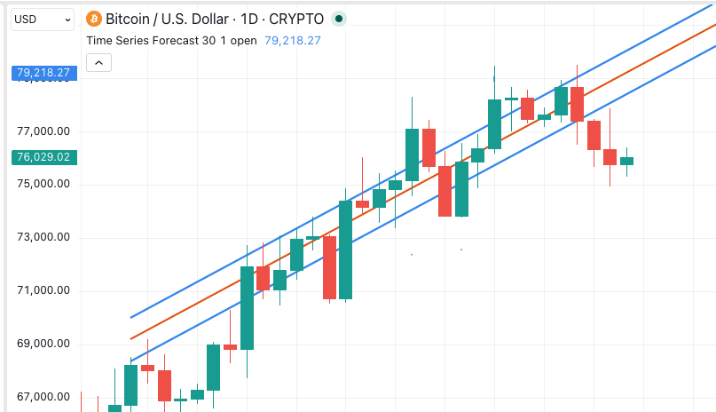
A Time Series Forecast trend strategy promises something most trend lines cannot: a line that leans ahead of price instead of trailing it. That speed is real. On three years of crypto candles, it was also the problem. The fastest version traded about 190 times a year, and fees turned a profit into a heavy loss.
This post shows what went wrong and how to give the indicator a job it can do. The rules below are hypotheses to test, not a recommendation.
How Does the Time Series Forecast Lean Ahead?
The Time Series Forecast (TSF) fits a straight best-fit line through the last N closing prices. This method is called linear regression. The TSF then extends that line one candle forward and plots the projected value. Our Time Series Forecast guide covers the calculation in full.
A moving average reports where price has been on average. The TSF reports where the recent slope says price should be next. In a steady trend, it sits close to price, or even ahead of it. That is why it reacts faster than an exponential moving average (EMA) of the same length.
The catch follows directly. A line that hugs price gets crossed by price constantly.
What Happened When Price Crossed the TSF?
We tested the textbook rule on Binance four-hour candles from November 2023 to November 2026. Hold a long position while the close sits above a 20-period TSF. Step aside when it closes below. We charged 0.1% per side and filled at the signal candle’s close. The first 200 candles were excluded as warm-up.
| Market, 4-hour | Entries per year | Return before fees | Return after 0.1% fees | Entries per year, close vs 20 EMA |
|---|---|---|---|---|
| BTC | 190 | +65.0% | -45.5% | 137 |
| ETH | 188 | +57.5% | -47.2% | 146 |
| SOL | 201 | +30.0% | -59.6% | 145 |
Hypothetical rule tests on past data, with no slippage. They are not trading results, and past behaviour may not repeat.
Before costs, the rule made money on all three markets. After costs, it lost roughly half the account on each. Nearly 200 round trips a year at 0.2% each adds up to about 38% of drag a year. The TSF also crossed more often than an EMA of the same length.
The lesson is not that the TSF lacks information. Its raw crossings are too frequent to pay for themselves.
Time Series Forecast Trend Strategy Rules to Test
The fix is to stop asking price to cross the TSF. Instead, use the TSF as the fast line against a slower average. Then add a broad trend filter.
Entry Conditions
Use four-hour candles. Generate a long entry signal when both hold on a completed candle:
- The 20-period TSF sits above the 50-period EMA.
- The close sits above the 200-period EMA.
The first condition reads the short-term trend. The second keeps the strategy out of long-term downtrends. Model fees and slippage on every fill.
Exit Conditions
Exit when either condition fails on a completed candle. The TSF drops below the 50-period EMA, or the close drops below the 200-period EMA.
You can add a protective stop at two times the 14-period Average True Range (ATR) below entry. ATR measures typical candle movement. Size each position from your loss budget and that stop distance.
The Control You Must Run
Swap the TSF for a 20-period EMA and keep everything else identical. This answers the only question that matters: does the forecast line add anything a plain average does not?
How Did the Filtered Version Compare?
We ran both versions on the same data, costs and fill rules. Buy-and-hold is shown for context.
| Market, 4-hour | TSF rule: return | TSF rule: max drawdown | EMA control: return | EMA control: max drawdown | Buy-and-hold: return |
|---|---|---|---|---|---|
| BTC | +38.3% | 25.8% | +58.3% | 28.6% | +73.1% |
| ETH | +99.2% | 40.5% | +80.8% | 44.4% | -5.2% |
| SOL | +66.1% | 44.4% | +199.1% | 39.3% | +16.3% |
Same assumptions as above: 0.1% fees per side, no slippage, hypothetical rules on past data.
Entries fell to about 33–38 a year, so fees stopped dominating. Both versions cut drawdown sharply against buy-and-hold. Max drawdown is the largest peak-to-trough fall in account value.
The head-to-head result is mixed. The TSF version beat its control on ETH, with a smaller drawdown. It trailed on BTC and SOL. It also traded about a third more often than the control on every market.
That is an honest finding, not a failure. Three markets cannot crown a winner. We tested one setting for each rule and did not tune either. Treat the table as a starting point for your own test.
Where Do TSF Backtests Go Wrong?
Ignoring costs. The first table is the clearest warning. A rule can look excellent before fees and lose heavily after them. Our guide to transaction cost modelling shows how to set realistic costs.
Reading the forecast as a target. The TSF projects the recent slope forward. It does not know about news, liquidations or a sell-off like the one on 5 November.
Shortening the period to get earlier signals. A shorter TSF hugs price even more tightly. That means more crossings and more fees.
Check the Comparison Itself
Skipping the control. Without the EMA version, a profitable TSF result tells you nothing about the TSF.
Tuning until it wins. Adjusting 20, 50 and 200 until the TSF beats the control is curve fitting. Log every combination you try, and read our post on the deflated Sharpe ratio.
Testing one regime. Our sample includes strong trends and long chop. Split your test into separate years and check each one.
Building the Time Series Forecast Strategy in Arrow Algo
The drag-and-drop visual builder expresses the filtered rule as a short chain of visual blocks:
- Add the exchange’s candle data and select the four-hour timeframe.
- Connect the close to a Time Series Forecast block, and set the period to 20.
- Connect the close to two EMA blocks, set to 50 and 200.
- Add a condition block that checks the TSF is above the 50-period EMA.
- Add a second condition block that checks the close is above the 200-period EMA.
- Join both with an AND condition block, then add a flat-position check.
- Connect the result to a buy action block. Under your rules, that block sends a signal.
- Build the exit as an OR of the two failed conditions into a sell action block.
Step through a few signals on the chart before trusting the totals. Then duplicate the strategy and replace the TSF block with a 20-period EMA block. Run both on the same data and the same fee settings.
No deployment is needed for any of this. If you later choose to deploy, your rules signal your own exchange account. The exchange decides whether to execute each order.
What Should You Take Into Your Own Test?
- The Time Series Forecast projects a regression line one candle ahead, so it hugs price closely.
- Price crossing a 20-period TSF triggered about 190 entries a year on four-hour crypto candles.
- Those crossings were profitable before fees and lost about half the account after them.
- Using the TSF as a fast line against a 50 EMA, with a 200 EMA filter, cut entries to under 40 a year.
- Against an identical EMA control, the TSF won on ETH and trailed on BTC and SOL. Run the control yourself.
Disclaimer: This content is for educational purposes only and does not constitute financial advice. Trading involves significant risk and you should only trade with capital you can afford to lose. Past performance is not indicative of future results. Always conduct your own research before making any trading decisions.
Ready to build your own automated trading strategies without writing a single line of code? Start for free at Arrow Algo and join thousands of traders who've made the switch to systematic trading.